NeRF

representing scenes as neural radiance fields for view synthesis

NeRF: Representing Scenes as Neural Radiance Fields for View Synthesis

Ben Mildenhall, Pratul P.Srinivasan, Matthew Tancik

paper :
https://arxiv.org/abs/2003.08934
project website :
https://www.matthewtancik.com/nerf
pytorch code :
https://github.com/yenchenlin/nerf-pytorch
https://github.com/csm-kr/nerf_pytorch?tab=readme-ov-file
tiny tensorflow code :
https://colab.research.google.com/github/bmild/nerf/blob/master/tiny_nerf.ipynb
referenced blog :
https://csm-kr.tistory.com/64
https://yconquesty.github.io/blog/ml/nerf/nerf_rendering.html#the-rendering-formula

코드 리뷰는 별도의 포스팅에 업로드하였습니다! Blog

핵심 요약 :

1. 여러 각도의 camera center에서 each input image pixel 방향으로 ray(r=o+td)를 쏜다.
2. ray를 discrete points로 sampling한다.
3. 3D coordinate x와 viewing direction d를 r(x)와 r(d)로 positional encoding한다.
4. r(x)를 MLP에 넣어 volume density를 얻고 여기에 r(d)까지 넣어 RGB color를 얻는다.
5. coarse network와 fine network(hierarchical sampling) 각각에서 volume density와 color를 이용한 volume rendering으로 ray마다 rendering pixel color를 구한다.

Introduction

Pipeline

• (a) march camera rays and generate sampling of 5D coordinates

• (b) represents volumetric static scene by optimizing continuous 5D function(fully-connected network)

1. input: single continuous 5D coordinate
   3D location \(x, y, z\)
   2D direction \(\theta, \phi\)
2. output:
   volume density (differential opacity) (how much radiance is accumulated by a ray)
   view-dependent RGB color (emitted radiance) \(c = (r, g, b)\)

• (c) synthesizes novel view by classic volume rendering techniques(differentiable) to accumulate(project)(composite) the color/density samples into 2D image along rays

• (d) loss between synthesized and GT observed images

Pipeline of NeRF architecture

Problem & Solution

Problem :

1. not sufficiently high-resolution representation
2. inefficient in the number of samples per camera ray

Solution :

1. input positional encoding for MLP to represent higher frequency function
2. hierarchical sampling to reduce the number of queries

Contribution

• represent continuous scenes as 5D neural radiance fields with basic MLP to render high-resolution novel views
• differentiable volume rendering + hierarchical sampling
• positional encoding to map input 5D coordinate into higher dim. space for high-frequency scene representation
• overcome the storage costs of discretized voxel grids by encoding continuous volume into network’s parameters
  => require only storage costs of sampled volumetric representations

Related Work

Neural 3D shape representation

• deep networks that map \(xyz\) coordinates to signed distance functions or occupancy fields
  => limit : need GT 3D geometry

• Niemeyer et al.
  => input : find directly surface intersection for each ray (can calculate exact derivatie)
  => output : diffuse color at each ray intersection location

• Sitzmann et al.
  => input : each 3D coordinate
  => output : feature vector and RGB color at each 3D coordinate
  => rendering by RNN that marches along each ray to decide where the surface is.

Limit : oversmoothed renderings, so limited to simple shapes with low geometric complexity

View synthesis and image-based rendering

• Given dense sampling of views, novel view synthesis is possible by simple light field sample interpolation

• Given sparser sampling of views, there are 2 ways :
  mesh-based representation and volumetric representation

• Mesh-based representation with either diffuse(난반사) or view-dependent appearance :
  Directly optimize mesh representations by differentiable rasterizers or pathtracers so that we reproject and reconstruct images

Limit :
gradient-based optimization is often difficult because of local minima or discontinuities or poor loss landscape
mesh 구조를 유지하면서 gradient-based optimization하는 게 어렵
needs a template mesh with fixed topology for initialization, which is unavailable in real-world

• Volumetric representation :
  well-suited for gradient-based optimization and less distracting artifacts
  train : predict a sampled volumetric representation (voxel grids) from input images
  test : use alpha-(or learned-)compositing along rays to render novel views
  (alpha-compositing : 아래 volume rendering section에서 설명 예정)
  CNN compensates discretization artifacts from low resolution voxel grids or CNN allows voxel grids to vary on input time

Limit :
good results, but limited by poor time, space complexity due to discrete sampling
\(\rightarrow\) discrete sampling : rendering high resol. image => finer sampling of 3D space

Author’s solution :
encode continuous volume into network’s parameters
=> higher quality rendering + require only storage cost of those sampled volumetric representations

Neural Radiance Field Scene Representation

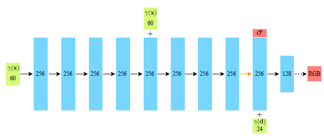
represent continuous scene by 5D MLP : (x, d) => (c, \(\sigma\))

Here, there are 2 key-points!

multiview consistent :
c is dependent on both x and d, but \(\sigma\) is only dependent on location x
3D coordinate x => 8 fc-layers => volume-density and 256-dim. feature vector

Lambertian reflection : diffuse(난반사) vs Specular reflection : 전반사

non-Lambertian effects : view-dependent color change to represent specular reflection
feature vector is concatenated with direction d => 1 fc-layer => view-dependent RGB color

Volume Rendering with Radiance Fields

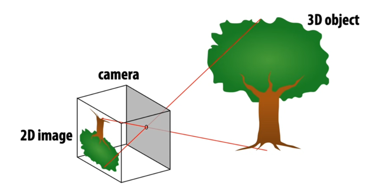
Ray from input image (pre-processing)

We use Ray to synthesize continuous-viewpoint images from discrete input images

\(r(t) = o + td\)
o : camera’s center of projection
d : viewing direction
t \(\in [ t_n , t_f ]\) : distance from camera center b.w. camera’s predefined near and far planes

How to calculate viewing direction d??

• 2D pixel-coordinate : \(\begin{bmatrix} x \\ y \\ 1 \end{bmatrix}\)
• 2D normalized-coordinate (\(z = 1\)) by intrinsic matrix :
  \(\begin{bmatrix} u \\ v \\ 1 \end{bmatrix}\) = \(K^{-1}\) \(\begin{bmatrix} x \\ y \\ 1 \end{bmatrix}\) = \(\begin{bmatrix} 1/f_x & 0 & -\frac{1}{f_x}\frac{W}{2} \\ 0 & 1/f_y & -\frac{1}{f_y}\frac{H}{2} \\ 0 & 0 & 1 \end{bmatrix}\) \(\begin{bmatrix} x \\ y \\ 1 \end{bmatrix}\)
  Since \(y, z\) have opposite direction between the real-world coordinate and pixel coordinate, we multiply (-1)
  \(\begin{bmatrix} u \\ v \\ 1 \end{bmatrix}\) = \(\begin{bmatrix} 1/f_x & 0 & -\frac{1}{f_x}\frac{W}{2} \\ 0 & -1/f_y & \frac{1}{f_y}\frac{H}{2} \\ 0 & 0 & -1 \end{bmatrix}\) \(\begin{bmatrix} x \\ y \\ 1 \end{bmatrix}\)
  Here, focal length in intrinsic matrix K is usually calculated using camear angle \(\alpha\) as \(\tan{\alpha / 2} = \frac{h/2}{f}\)
• 3D world-coordinate by extrinsic matrix :
  For extrinsic matrix \([R \vert t']\),
  \(o = t'\)
  \(d = R * \begin{bmatrix} u \\ v \\ 1 \end{bmatrix}\)
  Therefore, we can obtain \(r(t) = o + td\)

Volume Rendering from MLP output

We use differential classical volume rendering

Let ray \(r\) (traced through desired virtual camera) have near and far bounds \(t_n, t_f\)
expected color of ray \(r\) = \(C(r) = \int_{t_n}^{t_f} T(t) \sigma (r(t)) c(r(t), d) dt\)

• \(T(t) = \exp(- \int_{t_n}^{t} \sigma (r(s)) ds)\) : transmittance
  누적 값
  transmittance = 투과도 = CDF that a ray does not hit any particles from \(t_n\) to \(t\)
  투과도가 클수록, 시작점 \(t_n\)부터 현재 \(t\)까지 ray가 물체의 방해를 받지 않고 통과함
• \(\sigma (r(t))\) : volume density along the ray (learned by MLP)
  해당 지점에서의 값
  volume density = opacity = 불투명도 = extinction coefficient = alpha value for alpha-compositing
• \(c(r(t), d)\) : object’s color along the ray (learned by MLP)
  해당 지점에서의 값

volume rendering 식 유도 과정

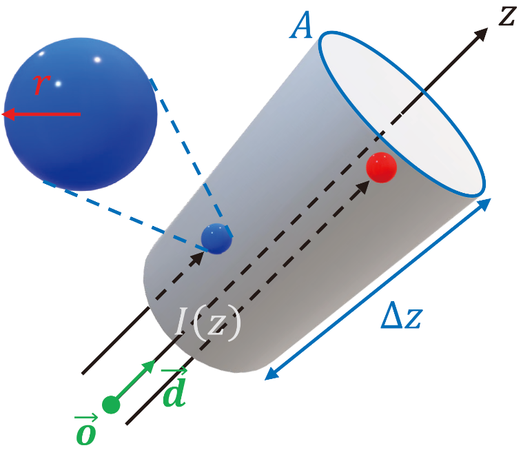
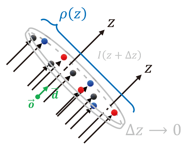
occluding objects are modeled as spherical particles with radius \(r\)
There are \(A \cdot \Delta z \cdot \rho (z)\)개의 particles in the slice where \(\rho (z)\) is particle density (the number of particles per unit volume)

Since solid particles do not overlap for \(\Delta z \rightarrow 0\),
\(A \cdot \Delta z \cdot \rho (z) \cdot \pi r^2\)만큼 area is occluded
즉, cross section \(A\)에서 \(\frac{A \cdot \Delta z \cdot \rho (z) \cdot \pi r^2}{A} = \pi r^2 \cdot \rho (z) \cdot \Delta z\)의 비율만큼 occluded

If \(\frac{A \cdot \Delta z \cdot \rho (z) \cdot \pi r^2}{A}\)만큼 rays are occluded, the light intensity decreases as
\(I(z + \Delta z) = (1 - \pi r^2 \rho (z) \Delta z) \times I(z)\)

Then the light density difference \(\Delta I = I(z + \Delta z) - I(z) = - \pi r^2 \rho (z) \Delta z \cdot I(z)\)
즉, \(dI(z) = - \pi r^2 \rho (z) I(z) dz = - \sigma (z) I(z) dz\)
where volume density (or opacity) is \(\sigma(z) = \pi r^2 \rho (z)\)
It makes sense because particle area와 particle density(particle 수)가 클수록 ray 감소량 (volume density)이 커지기 때문
ODE 풀면, \(I(z) = I(z_0)\exp(- \int_{z_0}^{z} \sigma (r(s)) ds)\)

Let’s define transmittance \(T(z) = \exp(- \int_{z_0}^{z} \sigma (r(s)) ds)\)
where \(I(z) = I(z_0)T(z)\) means the remainning intensity after rays travel from \(z_0\) to \(z\)
where transmittance \(T(z)\) means CDF that a ray does not hit any particles from \(z_0\) to \(z\)

If a ray passes empty space, there is no color
If a ray hits particles, there exists color (radiance is emitted)
Let’s define \(H(z) = 1 - T(z)\), which means CDF that a ray hits particles from \(z_0\) to \(z\)
CDF를 미분하면 PDF이므로
Then PDF is \(p_{hit}(z) = \frac{dH}{dz} = - \frac{dT}{dz} = \exp(- \int_{z_0}^{z} \sigma (r(s)) ds) \sigma (z) = T(z) \sigma (z)\)

Let a random variable \(R\) be the emitted randiance.
Then PDF \(p_R(ray) = P[R = c(z)] = p_{hit}(z) = T(z) \sigma (z)\)
Then the color of a pixel is expected radiance for ray bounded from \(t_n\) to \(t_f\)
\(C(ray) = E[R] = \int_{t_n}^{t_f} R \cdot p_R dz = \int_{t_n}^{t_f} c \cdot p_{hit} dz = \int_{t_n}^{t_f} T(z) \sigma (z) c(z) dz\)

\(t_n, t_f = 0., 1.\) for scaled-bounded and front-facing scenes after conversion to NDC (normalized device coordinates)
NDC에 대한 설명은 따로 정리한 블로그 글 How NDC Works? 참고

To apply the equation to our model by numerical quadrature,
we have to sample discrete points from continuous ray

Instead of deterministic quadrature(typically used for rendering voxel grids, but may limit resolution),
author divides a ray \(\left[t_n, t_f\right]\) into N = 64 bins(intervals), and chooses one point \(t_i\) for each bin by uniform sampling
\(t_i\) ~ \(U \left[t_n + \frac{i-1}{N}(t_f - t_n), t_n + \frac{i}{N}(t_f - t_n)\right]\)

Although we use discrete N samples, stratified sampling(층화 표집) enables MLP to be evaluated at continuous positions by optimization

Discretized version for N samples by Numerical Quadrature :
expected color \(\hat{C}(r) = \sum_{i=1}^{N} T_i (1 - \exp(- \sigma_{i} \delta_{i})) c_i\)

• \(\hat{C}(r)\) : differentiable about (\(\sigma_{i}, c_i\))
• \(\delta_{j} = t_{j+1} - t_j\) : the distance between adjacent samples
• \(T(t) = \exp(- \int_{t_n}^{t} \sigma (r(s)) ds) ~~ \rightarrow ~~ T_i = \exp(- \sum_{j=1}^{i-1} \sigma_{j} \delta_{j})\) where T_1 = 1
• \(\sigma (r(t)) dt ~~ \rightarrow ~~ \sigma_{j} \delta_{j} = 1 - \exp(-\sigma_{j} \delta_{j})\) by Taylor Series Expansion
• \[c(r(t), d) ~~ \rightarrow ~~ c_i\]

또는

\(p_{hit}(z_i) = \frac{dH}{dz} |_{z_i} ~~ \rightarrow ~~ H(z_{i+1}) - H(z_i) = (1 - T(z_{i+1})) - (1 - T(z_i)) = T(z_i) - T(z_{i+1}) = e^{- \sum_{j=1}^{i-1} \sigma_{j} \delta_{j}} - e^{- \sum_{j=1}^{i} \sigma_{j} \delta_{j}} = T(z_i)(1 - e^{- \sigma_{i} \delta_{i}})\)
Then the color of a pixel is expected radiance for ray bounded from \(t_n\) to \(t_f\)
\(\hat{C}(ray) = E[R] = \int_{t_n}^{t_f} R \cdot p_R dz ~~ \rightarrow ~~ \sum_{i=1}^{N} c_i \cdot p_{hit}(z_i) dz = \sum_{i=1}^{N} c_i T_i (1 - \exp(- \sigma_{i} \delta_{i}))\)

Final version :
expected color \(\hat{C}(r) = \sum_{i=1}^{N} T_i \alpha_{i} c_i\)
where \(T_i = \prod_{j=1}^{i-1} (1-\alpha_{j})\) and \(\alpha_{i} = 1 - \exp(-\sigma_{i} \delta_{i})\)
which reduces to traditional alpha-compositing problem

이 때, this volume rendering 식은 differentiable하므로 end-to-end learning 가능!!
a sequence of samples \(\boldsymbol t = {t_1, t_2, \ldots, t_N}\)에 대해
\(\frac{d\hat{C}}{dc_i} |_{\boldsymbol t} = T_i \alpha_{i}\) \(\frac{d\hat{C}}{d \sigma_{i}} |_{\boldsymbol t} = c_i \times (\frac{dT_i}{d \sigma_{i}} \alpha_{i} + \frac{d \alpha_{i}}{d \sigma_{i}} T_i) = c_i \times (0 + \delta_{i}e^{-\sigma_{i}\delta_{i}} T_i) = \delta_{i} T_i c_i e^{- \sigma_{i} \delta_{i}}\)

alpha-compositing :
여러 frame을 합쳐서 하나의 image로 합성하는 과정으로, 각 frame pixel마다 alpha 값(불투명도 값)(0~1)이 있어 겹치는 부분의 pixel 값을 결정

By divide-and-conquer approach (tail recursion),
\(c = \alpha_{1}c_{1} + (1 - \alpha_{1})(\alpha_{2}c_{2} + (1 - \alpha_{2})(\cdots)) = \alpha_{1}c_{1} + (1 - \alpha_{1})\alpha_{2}c_{2} + (1 - \alpha_{1})(1 - \alpha_{2})(\cdots) = \cdots = \sum_{i=1}^{N}(\alpha_{i}c_{i}\prod_{j=1}^{i-1}(1-\alpha_{j}))\) where \(\alpha_{0} = 0\)

If \(\alpha_{i} = 1 - \exp(-\sigma_{i} \delta_{i})\),
NeRF volume rendering 식 \(\hat{C}(r) = \sum_{i=1}^{N} T_i \alpha_{i} c_i\)과
alpha-compositing 식 \(c = \sum_{i=1}^{N}(\alpha_{i}c_{i}\prod_{j=1}^{i-1}(1-\alpha_{j}))\)은
SAME!!

Optimizing a Neural Radiance Field

Positional encoding (pre-processing)

kernel regression(dot product 및 더하기)을 사용하는 MLP의 특성상
If we use input directly, MLP is biased to learn low-frequency function (oversmoothed appearance) (no detail) (spectral bias)
So, low dim. input의 작은 변화에 대해 급격하게 변화하는 high-frequency output은 학습 잘 못함

Here, fourier features (sinusoidal signal은 input signal을 orthogonal space에서 표현 가능) let MLP learn high-frequency function in low-dim. domain [1]
If we map input into higher dim. space which contains both low and high frequency info. by fourier features, MLP can fit data with high-frequency variation
Due to positional encoding, MLP can behave as interpolation function where \(L\) determines the bandwidth of the interpolation kernel [1]
\(r : R \rightarrow R^{2L}\)
\(r(p) = (sin(2^0\pi p), cos(2^0\pi p), \cdots, sin(2^{L-1}\pi p), cos(2^{L-1}\pi p))\)
\(L=10\) for \(r(x)\) where x has three coordinates
\(L=4\) for \(r(d)\) where d has three components of the cartesian viewing direction unit vector

추가로, low-dim. input 정보를 high-frequency output에 반영하기 위해서는 kernel을 거친 뒤에도 orthogonal eigenvalue들이 많이 살아있어야 하는데 stationary kernel 또는 Spherical Harmonics가 이러한 역할 수행 가능

Hierarchical volume sampling

Densely evaluating N points by stratified sampling is inefficient
=> We don’t need much sampling at free space or occluded regions
=> Hierarchical sampling enables us to allocate more samples to regions we expect to contain visible content

We simultaneously optimize 2 networks with different sampling : coarse and fine

coarse sampling \(N_c\)개 : 위에서 배웠던 내용
author divides a ray into \(N_c\) = 64 bins(intervals), and chooses one point \(t_i\) for each bin by uniform sampling
\(t_i\) ~ \(U \left[t_n + \frac{i-1}{N_c}(t_f - t_n), t_n + \frac{i}{N_c}(t_f - t_n)\right]\)

fine sampling \(N_f\)개 : 새로운 내용
coarse sampling model’s output is a weighted sum of all coarse-sampled colors
\(\hat{C}(r) = \sum_{i=1}^{N_c} T_i \alpha_{i} c_i = \sum_{i=1}^{N_c} w_i c_i\)
where we define \(w_i = T_i \alpha_{i} = T_i (1 - \exp(-\sigma_{i} \delta_{i}))\) for \(i=1,\cdots,N_c\)
=> Given the output of coarse network, we try more informed (better) sampling where samples are biased toward the relevant parts of the scene volume
=> We sample \(N_f\)=128 fine points following a piecewise-constant PDF of normalized \(\frac{w_i}{\sum_{j=1}^{N_c} w_j}\)
=> Here, we use Inverse CDF Method for sampling fine points

Inverse transform sampling = Inverse CDF Method :
=> PDF (probability density function) : \(f_X(x)\)
=> CDF (cumulative distribution function) : \(F_X(x) = P(X \leq x) = \int_{-\infty}^x f_X(x) dx\)
idea : 모든 확률 분포의 CDF는 Uniform distribution을 따른다!
=> 따라서 CDF의 y값을 Uniform sampling하면, 그 y에 대응되는 x에 대한 (특정 PDF를 따르는) sampling을 구현할 수 있다!
=> 즉, CDF의 역함수를 계산할 수 있다면, 기본 난수 생성기인 Uniform sampling을 이용해서 확률 분포 X에 대한 sampling을 할 수 있다!
\(F_X(x)\) ~ \(U\left[0, 1\right]\)
\(X\) ~ \(F^{-1}(U\left[0, 1\right])\)
=> 이 때, CDF의 기울기가 가파를수록 그 곳에 물체가 있을 확률이 높다는 의미이며 Inverse CDF Method를 통해 더 많이 sampling됨

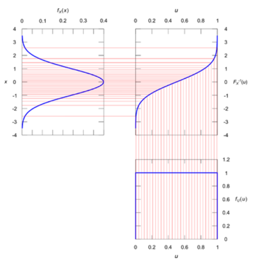
We evaluate coarse network using \(N_c\)=64 points per ray
We evaluate fine network using \(N_c+N_f\)=64+128=192 points per ray where we sample 128 fine points following PDF of coarse sampled points
In result, we use a total of 64+192=256 samples per ray to compute the final rendering color \(C(r)\)

Implementation details & Loss

1. Prepare RGB images, corresponding camera poses, intrinsic parameters and scene bounds (use COLMAP structure-from-motion package to estimate these parameters)
2. From H x W input image, randomly sample a batch of 4096 pixels
3. calculate continuous ray from each pixel \(r(t) = o + kd\)
4. coarse sampling of \(N_c\)=64 points per each ray \(t_i\) ~ \(U \left[t_n + \frac{i-1}{N_c}(t_f - t_n), t_n + \frac{i}{N_c}(t_f - t_n)\right]\)
5. positional encoding \(r(x)\) and \(r(d)\) for input
6. obtain volume density \(\sigma\) by MLP with \(r(x, y, z)\) as input
7. obtain color \(c\) by MLP with \(r(x, y, z)\) and \(r(\theta, \phi)\) as input
8. obtain rendering color of each ray by volume rendering \(\hat{C}(r) = \sum_{i=1}^{N} T_i (1 - \exp(- \sigma_{i} \delta_{i})) c_i\) from two networks ‘coarse’ and ‘fine’
9. compute loss
10. Adam optimizer with learning rate from \(5 \times 10^{-4}\) to \(5 \times 10^{-5}\)
11. optimization for a single scene typically takes around 100-300k iterations (1~2 days) to converge on a single NVIDIA V100 GPU

Here, we use L2 norm for loss
\(L = \sum_{r \in R} \left[{\left\|\hat{C_c}(r)-C(r)\right\|}^2+{\left\|\hat{C_f}(r)-C(r)\right\|}^2\right]\)
\(C(r)\) : GT pixel RGB color
\(\hat{C_c}(r)\) : rendering RGB color from coarse network : to allocate better samples in fine network
\(\hat{C_f}(r)\) : rendering RGB color from fine network : our goal
\(R\) : the set of all pixels(rays) across all images

Results

Datasets

Synthetic renderings of objects

• Diffuse Synthetic 360 : 4 Lambertian objects with simple geometry
• Realistic Synthetic 360 : 8 non-Lambertian objects with complicated geometry

Real images of complex scenes

• Real Forward-Facing : 8 scenes captured with a handheld cellphone

Measurement

• PSNR(Peak Signal-to-Noise Ratio) \(\uparrow\) : the ratio between the maximum possible power of a signal and the power of corrupting noise \(10\log_{10}\left(\frac{(MAX)^2}{MSE}\right)\)[dB]
• SSIM(Structural Similarity Index Map) \(\uparrow\) : compare image qualities in three ways: Lumincance(\(l\)), Contrast(\(c\)), Structural(\(s\))
  SSIM(x, y) = \([l(x,y)]^{\alpha}[c(x,y)]^{\beta}[s(x,y)]^{\gamma}=\frac{(2\mu_{x}\mu_{y}+C_1)(2\sigma_{xy}+C_2)}{(\mu_{x}^2+\mu_{y}^2+C_1)(\sigma_{x}^2+\sigma_{y}^2+C_2)}\) where \(l(x,y)=\frac{(2\mu_{x}\mu_{y}+C_1)}{\mu_{x}^2+\mu_{y}^2+C_1}\) and \(c(x,y)=\frac{(2\sigma_{x}\sigma_{y}+C_2)}{\sigma_{x}^2+\sigma_{y}^2+C_2}\) and \(s(x,y)=\frac{\sigma_{xy}+C_3}{\sigma_{x}\sigma_{y}+C_3}\)
  SSIM calculator :
  https://darosh.github.io/image-ssim-js/test/browser_test.html
• LPIPS \(\downarrow\)

Comparisons

• Neural Volumes (NV) :
  It synthsizes novel views of objects that lie entirely within a bounded volume in front of a distinct background.
  It optimizes 3D conv. network to predict a discretized RGB\(\alpha\) voxel grid and a 3D warp grid.
  It renders novel views by marching rays through the warped voxel grid
• Scene Representation Networks (SRN) :
  It represents continuous scene as an opaque surface.
  MLP maps each 3D coordinate to a feature vector, and we optimize RNN to predict the next step size along the ray using the feature vector.
  The feature vector from the final step is decoded into a color for that point on the surface. Note that SRN is followup to DeepVoxels by the same authors.
• Local Light Field Fusion (LLFF) :
  designed for producing novel views for well-sampled forward facing scenes
  trained 3D conv. network directly predicts a discretized frustum-sampled RGB\(\alpha\) grid (multiplane image), and then renders novel views by alpha-compositing and blending

Test for scenes from author's new synthetic dataset

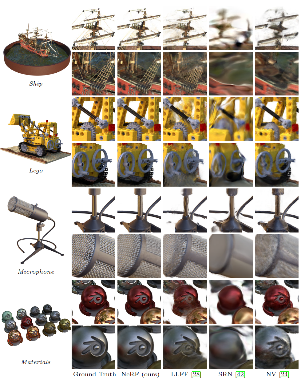
LLFF exhibits banding and ghosting artifacts
SRN produces blurry and distorted renderings
NV cannot capture the details
NeRF captures fine details in both geometry and appearance

Test for read-world scenes

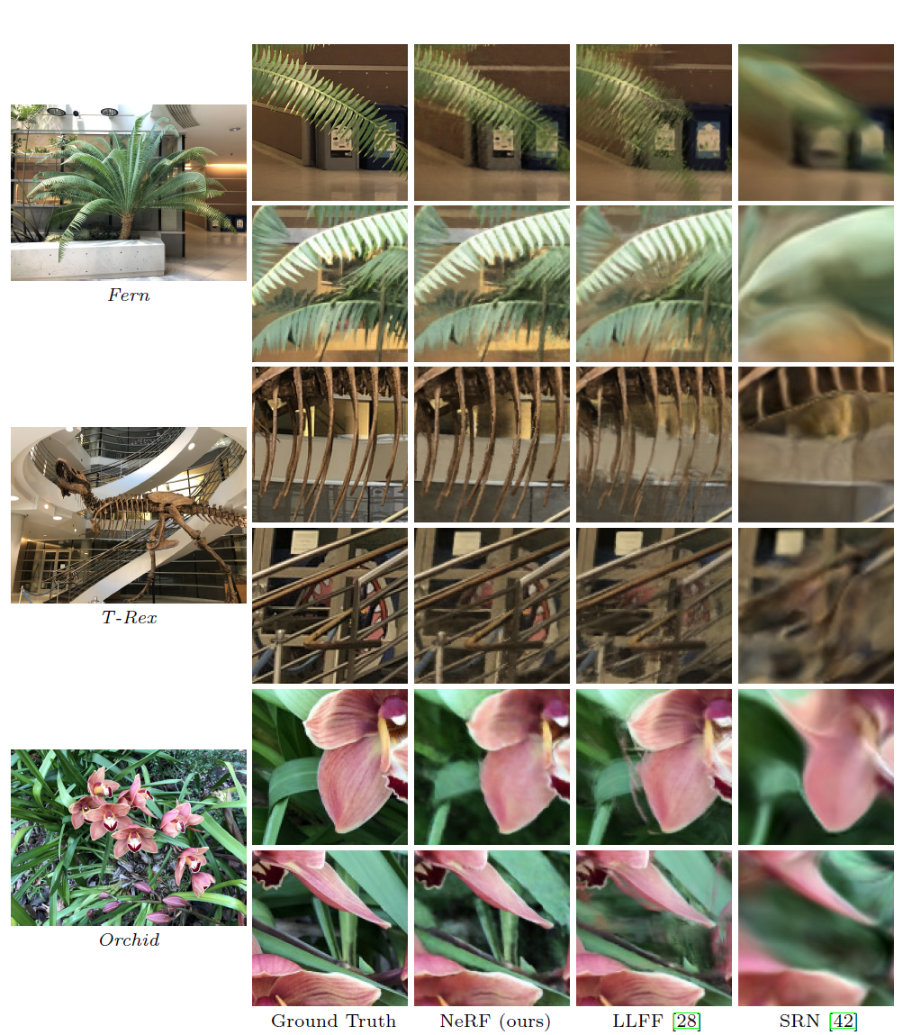
LLFF may have repeated edges because of blending between multiple renderings
NeRF also correctly reconstruct partially-occluded regions
SRN does not capture any high-frequency fine detail

Discussion

Ablation Studies

Conclusion

prior : MLP outputs discretized voxel representations
author : MLP outputs volume density and view-dependent emitted radiance

Future Work

efficiency :
Rather than hierarchical sampling, there is still much more progress to be made for efficient optimization and rendering of neural radiance fields

interpretability :
voxel grids or meshes admits reasoning about the expected quality, but it is unclear to analyze these issues when we encode scenes into the weights of MLP