Introduction

The Increasing Demand for Deep-learning Model Efficiency

In the area of deep learning, where neural networks have remarkable capabilites to learn complex patterns from massive datasets, there has emerged an ongoing pursuit for model efficiency. We need to achieve quick inference speed and less memory consumption in order to apply our deep-learning models to a wider range of users and applications. Especially, there is an increasing demand for deploying our models on mobile devices or edge devices and running the models in real-time, but the devices have resource-constrained hardware. Therefore it became important to strike a balance between model accuracy and computational cost.

Some Ways to Achieve Faster Inference Speed

There are several ways to achieve faster inference speed of deep-learning model.

Hardware accelerators : There are specialized hardware accelerators such as GPUs and TPUs which can be utilized to efficiently execute optimized deep-learning operations. We can achieve faster inference speed because the hardware accelerators are designed to utilize multi-threading or mult-processing to parallelize inference across multiple cores.
Optimized kernels : Kernel optimization refers to the process of improving the performance of codes that form the core computational operations of a software application. There are optimized kernels such as cuDNN and Intel MKL-DNN to perform optimized deep-learning operations. For example, we can achieve faster inference speed by vectorization or hardware-specific assembly-level optimization.
Model architecture : We can make a model of compact architecture such as NasNet, MobileNet, and FBNet. The models have more suitable architectures to deploy on mobile devices. Another example is that we can reduce computation by using bottleneck architecture like depth-wise separable convolution. By separating depth-wise convolution(= per channel convolution) and point-wise convolution(= 1x1 convolution), we extract many feature maps(as much as output channels) only at point-wise convolution with reduced computation. Eventually, we can reduce the number of parameters by about kernel_size x kernel_size times and we can achieve faster inference speed.
Model network optimization : We can optimize the existing model architecture via some optimization techniques. For example, we can reduce computation by pruning unnecessary layers, channels, or filters, which results in faster inference speed.
Quantization : We can optimize the existing model via reducing the precision of weights or activations. For example, we can reduce inference time and model size by quantizing weights or activations into lower bit-width.

The Reason why Quantization can be a Powerful Technique among them

It should be considered that the real world’s environment, on which our model is deployed, has limited resources. In real world, we cannot produce model with expensive hardware in large quantities, so we have to fix hardware at a proper price. Then our goal is to fit our model to the specific target hardware, usually for edge devices. In the case of kernel optimization, it has diminishing returns : Improving inference speed by optimizing computational operations in kernel can become increasingly difficult and may require more effort for relatively minor gains in performance. It’s because bottlenecks would exist at higher level such as I/O operations. Also, let us assume that we already designed the architecture of efficient small model as a backbone, but we need more improvement in inference time and model size.

How can we improve a existing model with fixed hardware, kernel, and model architecture? In that case, eventually quantization can be a powerful technique for inference speedup. Since quantization is lossy compression, it is important to achieve inference speedup with minimal accuracy drop.

A Brief Explanation of Quantization

Quantization is the process of reducing the precision of numerical values in neural network model : for example, from FP32 to INT8. By reducing the precision of weights or activations of deep-learning model, we can compress the model’s size and computational cost.

We will discuss how quantization works and look through various quantization techniques such as Post-Training-Quantization and Quantization-Aware-Training. In addition, we are also going to discuss how we quantize a model on different frameworks such as Pytorch and ONNX.

Nowadays, it is important to consider the balance between model accuracy and computational cost. By understanding the process of quantization, you will have the knowledge to use its potential and may efficiently bridge the gap between powerful AI models and resource-constrained real-world environments.

Method

Quantization

Overview of Quantization

In general, we use FP32 (= 32-bit floating-point) representation in deep-learning models because it provides a high level of numerical precision at the backpropagation during the training phase. However, performing operations in high bit-depth can be slow during the inference phase when it is deployed on the small device with resource-constrained hardware.

In the real world’s environment with resource-constrained hardware, we need small model size, small RAM bandwidth, and inference speedup with less accuracy drop. To achieve this goal, quantization can be a powerful technique.

Quantization is to perform computation and storage at reduced precision using lower bits.

We can quantize a model from FP32 to FP16, INT8, or INT4. Here, INT8 (= 8-bit integer) quantization is a common choice due to a balance between accuracy drop and efficiency improvement. By INT8 quantization, we can also utilize the advantages of modern specialized hardware accelerators such as NVIDIA GPU, TPU, and Qualcomm DSP so that they perform efficient INT8 arithmetic operations. If you quantize a model from FP32 to INT8, model size is typically reduced by 4 times and inference speed is improved by 2~4 times and required memory bandwidth is reduced by 2~4 times.

Principle of Quantization

Let me explain the main principle of quantization.

First, we specify the float range to be quantized and clip values outside the range.

Then we take the quantization equation \(x_q=clip(round({x\over s})+z)\) for the Quantization Layer and the dequantization equation \(x=s(x_q-z)\) for the Dequantization Layer.

Here, s is a scale factor which determines the range mapping and z is a zero-point integer such that \(x=0\) in FP32 corresponds to \(x_q=z\) in INT8.

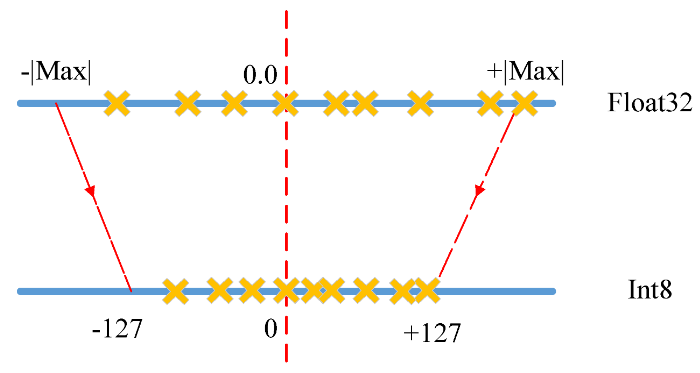
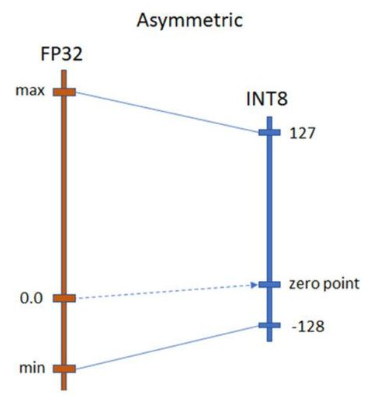
When we quantize weights or activations of a model by the above equation in the case of INT8 quantization, we have to map the range of FP32 precision into the range of INT8 precision as shown in the picture below.

Scale Quantization (Symmetric) from FP32 to IN8 vs Affine Quantization (Asymmetric) from FP32 to INT8

There are two types of range-mapping techniques in quantization according to the way of choosing scale factor s and zero-point integer z.

Affine Quantization Mapping : INT8 range is from -128 to 127, which is asymmetric.
\[s = \frac{\left| \beta\ - \alpha \right|}{2^{bit}-1}, z = - round(\frac{\alpha}{s})-2^{bit-1}\]
\(\alpha, \beta\) = min, max of original weight/activation values

\(\alpha_q, \beta_q\) = min, max of quantized weight/activation values ( \(\beta_q-\alpha_q=2^{bit}-1\) )
- advantage : Affine quantization generally offers tighter clipping range since \(\alpha,\ \beta\) are assigned to min, max of observed values itself. This can result in good quantization resolution. Also, it is particularly useful for quantizing non-negative activations of which distribution is not symmetric around zero. You can calibrate the zero-point integer to match the data distribution in order to reduce quantization errors.
- disadvantage : Affine quantization needs extra computations with calibration of zero-point integer and requires hardware-specific tweaks.
Scale Quantization Mapping : INT8 range is from -127 to 127, which is symmetric.
\[s = {\left| \beta \right| \over 2^{bit-1}-1}, z=0\]
\(\beta, \beta\) = min, max of original weight/activation values where \(\vert \alpha \vert \leq \vert \beta \vert\)

\(\beta_q, \beta_q\) = min, max of quantized weight/activation values (\(\beta_q = 2^{bit-1}-1\))
- advantage : Symmetric quantization eliminates the need to calculate zero-point integer and it is simpler than asymmetric quantization. Thus, symmetric quantization is more hardware-friendly and produces higher speedup.
- disadvantage : For skewed signals like non-negative activations, this can result in bad quantization resolution because the clipping range includes negative values that never show up in the input.

To quantize each layer by MinMax, we need to know the value of \(\alpha,\ \beta\) to determine scale factor s and zero-point integer z. Thus, we insert observer into each layer of a model and the observers gather statistics from the activations and weights of a neural network during the forward pass of calibration process. These statistics are then used to determine scale-factor and zero-point integer.

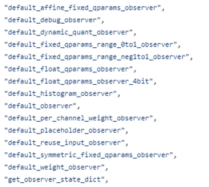
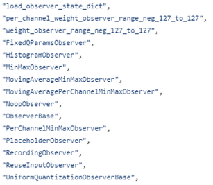
The above equations are based on MinMax observer, but there are also many other observers in Pytorch framework as shown in the picture below.

Different observers to determine scale factor and zero-point integer

Types of Quantization

Quantization techniques can be grouped into two classes depending on to which stages of neural network model’s development pipeline they are applicable. One is PTQ (Post-Training Quantization) which is applicable after training is finished. The other is QAT (Quantization-Aware Training) which is applicable during training.

PTQ (Post-Training Quantization) : It is to quantize a model which was already trained in high precision. The quantization has nothing to do with training.

If the clipping range of activation is determined during inference, it is called Post-Training Dynamic Quantization.

If the clipping range of activation is determined before inference, it is called Post-Training Static Quantization.
QAT (Quantization-Aware Training) : It is to fine-tune a model with integrating the quantization effects. The model is exposed to quantization during training by inserting observers and fake-quantization modules(e.g. QuantStub and DeQuantStub) in the forward/backward-pass. Here, fake-quantization modules mimic the behavior of quantized operations while working with full precision representations, allowing developers to simulate the effects of quantization during training and evaluation.

QAT is more complicated than PTQ since it needs training process. However, QAT outperforms PTQ since the weights of the model is fine-tuned to the quantization task. Therefore, QAT may be an appropriate method for small models such as MobileNet since small models on edge device are more sensitive to quantization error.

Model Fusion

In addition, we usually fuse modules of a model before quantization since it would have less accuracy drop : typically Conv2d-BatchNorm or Conv2d-ReLU or Conv2d-BatchNorm-ReLU or Linear-ReLU. It’s because the overall number of layers to be quantized and the number of operations are reduced if you fuse modules. This reduction of quantization overhead can mitigate the cumulative quantization error, resulting in a less accuracy drop.

code implementation with torch.ao.quantization library

# One Example of Model Fusion : timm resnet18
# torch.ao.quantization.fuse_modules() is used     for PTQ
# torch.ao.quantization.fuse_modules_qat() is used for QAT
 
torch.ao.quantization.fuse_modules_qat(model, [["conv1", "bn1", "act1"]], inplace=True)

for name1, module1 in model.named_children():
    if "layer" in name1 and module1 is not None:
        for name2, module2 in module1.named_children():
            torch.ao.quantization.fuse_modules_qat(module2, [["conv1", "bn1"], ["conv2", "bn2"]], inplace=True)
            for name3, module3 in module2.named_children():
                if name3 == "downsample" and module3 is not None:
                    torch.ao.quantization.fuse_modules_qat(module3, [["0", "1"]], inplace=True)

Post-Training Dynamic Quantization in Pytorch

If the clipping range of activation is determined during inference, it is called dynamic quantization. Only weights of a trained model are quantized before inference and activations of the model should be quantized dynamically during inference. So, observer which can compute quantization parameters in real-time manner should be used such as MinMax and Percentile.

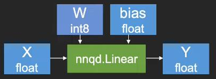
Post-Training Dynamic Quantization

advantage :

Inference accuarcy may be higher than Static Quantization since scale factor and zero-point integer of activations are determined in real-time during inference such that they fit our input data.

Post-Training Dynamic Quantization is appropriate to dynamic models like LSTMs or BERT. It’s because the disbribution of activation values of dynamic models can vary significantly depending on the input data.
disadvantage :

The scale factor and zero-point integer of activations should be computed dynamically at inference runtime. This results in the increase of the cost of inference and has less improvement of inference latency than Static Quantization.

Note that inference of a quantized model is still executed on CPU for Pytorch framework. (For other frameworks, GPU may work.)

code implementation with torch.ao.quantization library

It is very simple to implement Post-Training Dynamic Quantization as shown below.

You can specify submodules which will be quantized using “qconfig_spec” argument.

That’s all!

quantized_model = torch.ao.quantization.quantize_dynamic(model, qconfig_spec={torch.nn.Linear}, dtype=torch.quint8)

Post-Training Static Quantization in Pytorch

If the clipping range of activation is determined before inference, it is called static quantization. Both weights and activations of a trained model are quantized before inference. Here, by calibration, observers observe the range of stored values to determine quantization parameters.

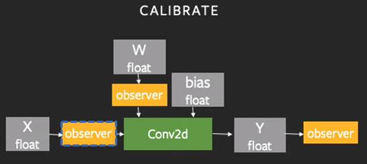
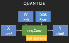
Post-Training Static Quantization - calibrate & quantize

advantage :

It is relatively easy to find scale factor and zero-point integer in advance before inference.

Post-Training Static Quantization is appropriate to CNN models since their throughput is limited by memory bandwidth for activations and we can figure out the disbribution of activation values of CNN models during calibration.
disadvantage :

Smaller model like Mobile CNN is more sensitive to quantization errors, so Post-Training Quantization may have significant accuracy drop. It’s the moment when we need Quantization-Aware Training.

Note that inference of a quantized model is still executed on CPU for Pytorch framework. (For other frameworks like tflite, both CPU and GPU may work.)

code implementation with torch.ao.quantization library

Step 1. Module Fusion :

Fuse modules for less accuracy drop

torch.ao.quantization.fuse_modules(model, [["conv1", "bn1", "act1"]], inplace=True)

for name1, module1 in model.named_children():
    if "layer" in name1 and module1 is not None:
        for name2, module2 in module1.named_children():
            torch.ao.quantization.fuse_modules(module2, [["conv1", "bn1"], ["conv2", "bn2"]], inplace=True)
            for name3, module3 in module2.named_children():
                if name3 == "downsample" and module3 is not None:
                    torch.ao.quantization.fuse_modules(module3, [["0", "1"]], inplace=True)

# insert torch.ao.quantization.QuantStub() layer 
#	and torch.ao.quantization.DeQuantStub() layer 
# at the beginning and end of forward() respectively.

Step 2. Prepare :

Insert observer and prepare the quantization process

# 'x86' or 'fbgemm' for server inference
# 'qnnpack' for mobile inference
torch.backends.quantized.engine = 'fbgemm' 
model.qconfig = torch.ao.quantization.get_default_qconfig('fbgemm')
# You can use different observers for quantized_model.qconfig
torch.ao.quantization.prepare(model, inplace=True)

Step 3. Calibration :

Forward-pass to determine the scale factor and zero-point integer based on the given input calibration dataset.

# forward pass of model in .eval() phase
# observer computes scale factor and zero-point integer by calibration
model.eval()
model.to(torch.device("cpu:0"))
for i, (img, gt) in enumerate(calibrate_loader):
		img = img.to(torch.device("cpu:0"))
		gt = gt.to(torch.device("cpu:0"))
	  model(img)

Step 4. Convert :

Convert from FP32 to reduced precision based on the calibrated quantization parameters

torch.ao.quantization.convert(model, inplace=True)

code implementation with pytorch_quantization library

Step 1. Initialize quantizable modules :

pytorch_quantization library supports only the quantization of the layers shown below.

QuantConv1d, QuantConv2d, QuantConv3d, QuantConvTranspose1d, QuantConvTranspose2d, QuantConvTranspose3d
QuantLinear
QuantAvgPool1d, QuantAvgPool2d, QuantAvgPool3d, QuantMaxPool1d, QuantMaxPool2d, QuantMaxPool3d

If you want to quantize another layer, you should implement the quantized version of custom modules. (In my case, I implemented QuantHardswish and QuantConvReLU2d.)

For the model instance that you create after quant_modules.initialize(), it automatically converts the default modules and custom modules into their quantizable version via monkey-patching.

Limitation : pytorch_quantization library “immediately” converts the modules of a model into their quantized version as soon as the model is loaded after quant_modules.initialize(). Therefore the modules to be quantized must be the modules of a model to be loaded.

from pytorch_quantization import quant_modules

custom_quant_modules = [(nn, "Hardswish", QuantHardswish), 
		(torch.ao.nn.intrinsic.modules.fused, "ConvReLU2d", QuantConvReLU2d)]
quant_modules.initialize(custom_quant_modules=custom_quant_modules)

# create a model instance
# then modules are substituted into quantizable version 
# automatically via monkey-patching

Step 2. Prepare :

I utilized histogram-based calibration for activations, but you can also try another calibration method.

quant_desc_input = QuantDescriptor(calib_method='histogram')
quant_nn.QuantConv2d.set_default_quant_desc_input(quant_desc_input)
quant_nn.QuantLinear.set_default_quant_desc_input(quant_desc_input)
QuantHardswish.set_default_quant_desc_input(quant_desc_input)
QuantConvReLU2d.set_default_quant_desc_input(quant_desc_input)

Step 3. Calibration :

Forward-pass to determine the scale factor and zero-point integer

# If there is calibrator, disable quantization and enable calibrator
# Otherwise, disable the module itself
with torch.no_grad():
# Enable calibrators to collect statistics
for name, module in model.named_modules():
    if isinstance(module, quant_nn.TensorQuantizer):
        if module._calibrator is not None:
            module.disable_quant() # use full precision data to calibrate
            module.enable_calib()
        else:
            module.disable()

# Calibration  
for i, (image, ground_truth) in enumerate(data_loader):
    model(image.cuda()) # forward pass of model in .eval() phase
    if i >= 7:
        break

# If there is calibrator, enable quantization and disable calibrator
# Otherwise, enable the module itself
for name, module in model.named_modules():
    if isinstance(module, quant_nn.TensorQuantizer):
        if module._calibrator is not None:
            module.enable_quant()
            module.disable_calib()
        else:
            module.enable()

# After calibration, quantizers obtain amax set, which is
# absolute maximum input value representable in the quantized space
# In default, amax for weight is per channel 
#         and amax for activation is per tensor.
for name, module in model.named_modules():
    if isinstance(module, quant_nn.TensorQuantizer):
        if module._calibrator is not None:
            if isinstance(module._calibrator, calib.MaxCalibrator):
                module.load_calib_amax(strict=False)
            else:
                # method = "percentile" or "mse" or "entropy"
								module.load_calib_amax(method="percentile", 
									percentile=99.99, strict=False) 
				# You can check 
				print(F"{name:40}: {module}")		

QAT(Quantization-Aware Training) in Pytorch

It has similar steps with Post-Training Static Quantization, but the difference is that the weights of a model are updated via fine-tuning to quantization task. To emulate the quantization, we insert fake-quantization modules at the beginning and end of forward() function.

advantage :

The weights of model is updated to fit the quantization task (a.k.a fine-tuning), so it has usually higher accuracy than Post-Training Quantization.
disadvantage :

It needs additional resources due to training process, so it is more complicated.

Note that training of a model can be executed on both CPU and GPU, but inference of a quantized model is still executed on CPU for Pytorch framework. To compare the inference time(latency) between original model and quantized model, I did inference on CPU for both models.

code implementation using torch.ao.quantization library

Step 1. Module Fusion :

Fuse modules for less accuracy drop

torch.ao.quantization.fuse_modules_qat(model, [["conv1", "bn1", "act1"]], inplace=True)

for name1, module1 in model.named_children():
    if "layer" in name1 and module1 is not None:
        for name2, module2 in module1.named_children():
            torch.ao.quantization.fuse_modules_qat(module2, [["conv1", "bn1"], ["conv2", "bn2"]], inplace=True)
            for name3, module3 in module2.named_children():
                if name3 == "downsample" and module3 is not None:
                    torch.ao.quantization.fuse_modules_qat(module3, [["0", "1"]], inplace=True)

# To emulate the quantization process,
# insert torch.ao.quantization.QuantStub() layer 
#	and torch.ao.quantization.DeQuantStub() layer 
# at the beginning and end of forward() respectively.

Step 2. Prepare :

Insert observer and prepare the quantization process

# 'x86' or 'fbgemm' for server inference
# 'qnnpack' for mobile inference
torch.backends.quantized.engine = 'fbgemm'
model.qconfig = 
	torch.ao.quantization.get_default_qat_qconfig('fbgemm')
# You can use different observers for quantized_model.qconfig
torch.ao.quantization.prepare_qat(model.train(), inplace=True)

Step 3. Calibration + Fine-Tuning (Training) :

First, enable the observers and fake-quantization modules.

The observers and fake-quantization modules will compute the scale factor and zero-point integer during calibration.

Second, fine-tune the model until loss converges (training).

Here, note that you should finish the calibration around the beginning of epochs. So, disable the observers and freeze the BatchNorm stats around the beginning of epochs (epoch 4, 3 in my case) so that we can focus on updating the weights of the model with the observer’s fixed quantization parameters.

quantized_model.apply(torch.ao.quantization.enable_observer)
quantized_model.apply(torch.ao.quantization.enable_fake_quant)

for epoch in range(num_epochs):
	loss, acc = train_one_epoch(model, train_loader, criterion, optimizer, epoch)
	print("train loss : {.8f} acc : {:.5f}".format(loss, acc))
	
	loss, acc = test(model, test_loader, criterion, optimizer)
	print("test loss : {.8f} acc : {:.5f}".format(loss, acc))
	
	with torch.inference_mode():
		if epoch >= 4:
			quantized_model.apply(torch.ao.quantization.disable_observer)
		if epoch >= 3:
			quantized_model.apply(torch.nn.intrinsic.qat.freeze_bn_stats)

Step 4. Convert :

Convert from FP32 to reduced precision based on the calibrated quantization parameters

model = torch.ao.quantization.convert(model, inplace=False)

Quantization in ONNX

Definition of ONNX

ONNX(Open Neural Network Exchange) is an open standard to facilitate interoperability between different DNN frameworks.

Necessity of ONNX

Deploying models on specific hardware can be challenging due to the difference in hardware’s architecture and runtime environment. ONNX deals with this challenge by providing a standardized way to represent deep-learning models so that they can be easily transferred across various frameworks and easily deployed on specific hardware device. It bridges the gap between model development on framework and model deployment on hardware.

Framework-Agnostic : ONNX allows you to train deep-learning models in one framework such as PyTorch and TensorFlow, and then export them to the ONNX format. This enables you to choose the best framework which is familiar with you and suitable for the model development. And then you can deploy the model on different target hardware without extensive modifications.
Hardware Optimization : Different hardware have varying architectures and optimizations. Here, hardware-specific optimizations are incorporated into onnxruntime, so onnxruntime allows the model to take full advantage of the underlying hardware-specific capabilities and perform inference efficiently on the target device. In detail, ONNX Runtime works with different hardware acceleration libraries through its extensible hardware-specific Execution Providers listed below.

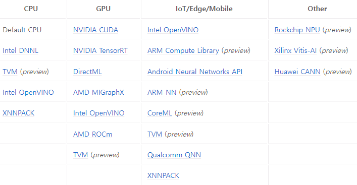
Inference in ONNX

You can perform forward-pass of an ONNX model following the code below.

code implementation using onnxruntime library

import onnxruntime

def benchmark(model_path):
    session = onnxruntime.InferenceSession(model_path)
    input_name = session.get_inputs()[0].name

    total = 0.0
    runs = 10
    input_data = np.zeros((1, 3, 224, 224), np.float32) # B, C, H, W
    # Warming up
    _ = session.run([], {input_name: input_data})
    for i in range(runs):
        start = time.perf_counter()
        _ = session.run([], {input_name: input_data})
        end = (time.perf_counter() - start) * 1000
        total += end
        print(f"{end:.2f}ms")
    total /= runs
    print(f"Avg: {total:.2f}ms")

Quantization in ONNX

Quantization in ONNX Runtime refers to INT8 or UINT8 linear quantization of an ONNX model. There are two ways to represent quantized ONNX models.

Operator-oriented (QOperator) :

All the quantized operators have their own ONNX definitions like QLinearConv and MatMulInteger.
Tensor-oriented (QDQ) :

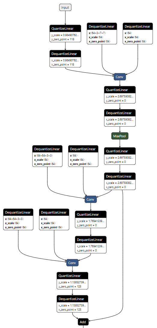
This format inserts <tensor - QuantizeLinear - DequantizeLinear> between the original operators to simulate the quantization and dequantization process. In the case of activations, QuantizeLinear layer is used for quantizing and DequantizeLinear layer is used for dequantizing respectively. In the case of weight, only DequantizeLinear layer is inserted.

In Dynamic Quantization, a ComputeQuantizationParameters functions proto is inserted to calculate quantization parameters on the fly. In Static Quantization, QuantizeLinear and DeQuantizeLinear operators carry the quantization parameters (scale factor and zero-point integer) of activations or weights.

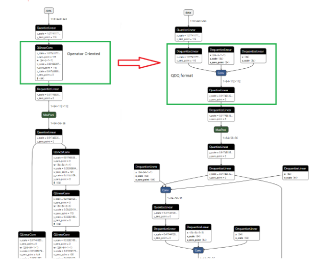
Visualization of ONNX model via netron.app Left : QOperator format of a quantized ONNX model Right : QDQ format of a quantized ONNX model

For more details, refer to the link below.

https://onnxruntime.ai/docs/performance/model-optimizations/quantization.html

code implementation using onnxruntime library (CPU, QDQ format)

I will introduce how to quantize an ONNX model using CPU hardware and QDQ format.

It follows the link below.

https://github.com/microsoft/onnxruntime-inference-examples/tree/main/quantization/image_classification/cpu

Step 1. Pre-process

Pre-processing is to prepare ONNX model for better quantization. It consists of three optional steps : Symbolic shape inference, Model optimization, and ONNX shape inference.

Both Symbolic shape inference and ONNX shape inference figure out the tensor shapes. Model optimization performs module fusion.

import onnxruntime
from onnxruntime.quantization.shape_inference import quant_pre_process

# whether you skip Model optimization since model size is greater than 2GB
parser.add_argument("--skip_optimization", default=False)

# whether you skip ONNX shape inference
parser.add_argument("--skip_onnx_shape", default=False)

# whether you skip Symbolic shape inference
parser.add_argument("--skip_symbolic_shape", default=False)

parser.add_argument("--auto_merge", default=False)
parser.add_argument("--int_max", default=2**31-1)
parser.add_argument("--guess_output_rank", default=False)
parser.add_argument("--verbose", default=0)
parser.add_argument("--save_as_external_data", default=False)
parser.add_argument("--all_tensors_to_one_file", default=False)
parser.add_argument("--external_data_location", default=None)
parser.add_argument("--external_data_size_threshold", default=1024)

quant_pre_process(
        input_onnxmodel_path,
        output_onnxmodel_path,
        args.skip_optimization,
        args.skip_onnx_shape,
        args.skip_symbolic_shape,
        args.auto_merge,
        args.int_max,
        args.guess_output_rank,
        args.verbose,
        args.save_as_external_data,
        args.all_tensors_to_one_file,
        args.external_data_location,
        args.external_data_size_threshold
)

Step 2. Quantize

Model optimization may also be performed during quantization by default for historical reasons. However, it’s highly recommended to perform model optimization during pre-process(Step 1) and turn off model optimization during quantization(Step 2) for the ease of debugging.

(i) Dynamic Quantization :

It calculates quantization parameters for activations dynamically

import onnxruntime
from onnxruntime.quantization import QuantFormat, QuantType, quantize_dynamic

# Tensor-oriented QDQ format of quantized ONNX model
parser.add_argument("--quant_format", default=QuantFormat.QDQ)

# You can use per-channel quantization if accuracy drop is significant
parser.add_argument("--per_channel", default=True)

# If accuracy drop is significant, it may be caused by saturation (clamped)
# Then you can try reduce_range
# reduce_range == True : quantize weights with 7-bits. 
#                        It may improve accuracy for non-VNNI machine
parser.add_argument("--reduce_range", default=True)

# nodes_to_exclude : specify nodes which you will freeze and will not quantize

quantize_dynamic(
        input_onnxmodel_path,
        output_onnxmodel_path,
        per_channel=args.per_channel,
        reduce_range=args.reduce_range,
        weight_type=QuantType.QInt8, 
        nodes_to_exclude=['/layer4/layer4.0/conv1/Conv', 
                          '/layer4/layer4.0/conv2/Conv', 
                          '/layer4/layer4.0/downsample/downsample.0/Conv',  
                          '/layer4/layer4.1/conv1/Conv', 
                          '/layer4/layer4.1/conv2/Conv',
                          '/fc/Gemm']
)

(ii) Static Quantization :

It calculates quantization parameters using calibration input data before inference.

ONNX Runtime quantization tool supports three calibration methods: MinMax, Entropy and Percentile.

ONNX Runtime quantization on CPU can run U8U8, U8S8, and S8S8. Here, U8S8 means that activation and weight are quantized to UINT8(unsigned) and INT8(signed) respectively. And S8S8 with QDQ is the default setting since it may have balance between performance and accuracy.

Note that S8S8 with QOperator will be slow on x86-64 CPUs and should be avoided in general. Also, note that ONNX Runtime quantization on GPU only supports S8S8.

import onnxruntime
from onnxruntime.quantization import QuantFormat, QuantType, quantize_static

# Tensor-oriented QDQ format of quantized ONNX model
parser.add_argument("--quant_format", default=QuantFormat.QDQ)

# You can use per-channel quantization if accuracy drop is significant
parser.add_argument("--per_channel", default=True

# If accuracy drop is significant, it may be caused by saturation (clamped)
# Then you can try reduce_range or U8U8
# reduce_range == True : quantize weights with 7-bits. 
#                        It may improve accuracy for non-VNNI machine
parser.add_argument("--reduce_range", default=True)

# nodes_to_exclude : specify nodes which you will freeze and will not quantize

# Create a set of inputs called calibration data
dr = resnet18_data_reader.ResNet18DataReader(
        calibration_dir_path, input_onnxmodel_path
    )

quantize_static(
        input_onnxmodel_path,
        output_onnxmodel_path,
        dr,
        quant_format=args.quant_format,
        per_channel=args.per_channel,
        reduce_range=args.reduce_range,
        activation_type=QuantType.QUInt8,
        weight_type=QuantType.Int8, 
        nodes_to_exclude=['/layer4/layer4.0/conv1/Conv', 
                          '/layer4/layer4.0/act1/Relu',
                          '/layer4/layer4.0/conv2/Conv', 
                          '/layer4/layer4.0/downsample/downsample.0/Conv', 
                          '/layer4/layer4.0/Add', 
                          '/layer4/layer4.0/act2/Relu', 
                          '/layer4/layer4.1/conv1/Conv', 
                          '/layer4/layer4.1/act1/Relu', 
                          '/layer4/layer4.1/conv2/Conv', 
                          '/layer4/layer4.1/Add', 
                          '/layer4/layer4.1/act2/Relu', 
                          '/global_pool/pool/GlobalAveragePool', 
                          '/global_pool/flatten/Flatten', '/fc/Gemm'],
        extra_options={'CalibMovingAverage':True, 'SmoothQuant':True}
)

Step 3. Debugging

Quantization is a lossy compression, so it may drop a model’s accuracy. To improve the problematic parts, you can compare the weights and activations tensors between the original computation graph and the quantized comptuation graph. By debugging, you can identify where they differ most and avoid quantizing these nodes using “nodes_to_exclude” argument in Step 2. Quantize.

from onnxruntime.quantization.qdq_loss_debug import (
	collect_activations, compute_activation_error, compute_weight_error,
	create_activation_matching, create_weight_matching,
	modify_model_output_intermediate_tensors)

# Comparing weights of float model vs qdq model
matched_weights = create_weight_matching(float_model_path, qdq_model_path)
weights_error = compute_weight_error(matched_weights)
for weight_name, err in weights_error.items():
  print(f"Cross model error of '{weight_name}': {err}\n")

# Augmenting models to save intermediate activations
modify_model_output_intermediate_tensors(float_model_path, aug_float_model_path)
modify_model_output_intermediate_tensors(qdq_model_path, aug_qdq_model_path)

# Running the augmented floating point model to collect activations
dr = resnet18_data_reader.ResNet18DataReader(
        calibration_dir_path, float_model_path
)
float_activations = collect_activations(aug_float_model_path, dr)

# Running the augmented qdq model to collect activations
dr.rewind()
qdq_activations = collect_activations(aug_qdq_model_path, dr)

# Comparing activations of float model vs qdq model
act_matching = create_activation_matching(qdq_activations, float_activations)
act_error = compute_activation_error(act_matching)
for act_name, err in act_error.items():
  print(f"Cross model error of '{act_name}': {err['xmodel_err']} \n")
  print(f"QDQ error of '{act_name}': {err['qdq_err']} \n")

Summary :

Assume that you implemented Step 1. into preprocess.py and Step 2. into quantize.py and Step 3. into debug.py with proper I/O. Then you can run them in terminal as shown below.

(i) If you do not optimize ONNX model during quantization (recommended)

# Step 1. Pre-process
python preprocess.py --input original.onnx --output preprocess.onnx
# Step 2. Quantize without optimization
python quantize.py --input preprocess.onnx --output quantized.onnx
# Step 3. Debug
python debug.py --float_model preprocess.onnx --qdq_model quantized.onnx

(ii) If you optimize ONNX model during quantization (default)

# Step 1. Pre-process
python preprocess.py --input original.onnx --output preprocess.onnx
# Step 2. Quantize with optimization
python quantize.py --input preprocess.onnx --output quantized_2.onnx
# Step 3. Debug
python preprocess.py --input original.onnx --output preprocess_2.onnx --skip_symbolic_shape True
python debug.py --float_model preprocess_2.onnx --qdq_model quantized_2.onnx

Result

shufflenetv2

Pytorch

Experiment

dataset :
calibration : batch_size = 32, iteration = 32
inference : batch_size = 128, iteration = 61
hardware : cpu

method	model size [MB]	inference time [s]	loss	ocualr_nme [%]	pupil_nme [%]
Original Model (partial fuse)	7.15	306.59	0.01121577	3.51807	4.87317
Original Model (all fuse)	7.01	227.92	0.01121577	3.51807	4.87317
Static PTQ calibrated with dummy input (partial fuse)	2.19	174.01	0.04872545	15.87943	21.99286
Static PTQ calibrated with our input dataset (partial fuse)	2.19	173.31	0.01834808	5.68243	7.87280
Static PTQ calibrated with our input dataset (all fuse)	2.01	161.74	0.01228440	3.83984	5.31811

Result

By Post-Training Static Quantization, model size of shufflenetv2 was reduced by about 3.5 times.
By Post-Training Static Quantization, inference speed was improved by about 1.5 times.
To minimize the accuracy drop, it is better to use our dataset as input of calibration rather than dummy input.

It’s because, during calibration, we can figure out the range of activations similarly to when the model was trained and inferred.
To minimize the accuracy drop, it is better to fuse all the layers of Conv-Bn or Conv-Bn-ReLU or Conv-ReLU because the number of layers to be quantized are reduced.

resnet18

Pytorch

Exp 1. QAT - The effect of learning rate

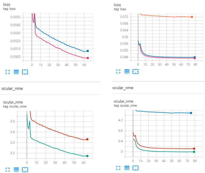
The proper learning rate of fine-tuning is lr = 1e-8 which is 0.1 times the learning rate of pre-trained model 1e-7.

I tested various values of learning rate to find the optimal value. For example, the left graph (lr = 1e-10) below shows underfitting and slow convergence due to small learning rate. However, the right graph (lr = 1e-8) below shows proper convergence.

loss graph

pink : test loss before quantization
blue : training loss before quantization
orange : test loss after quantization

nme graph

green : test nme before quantization
red : training nme before quantization
blue : test nme after quantization

left : lr = 1e-10
right : lr = 1e-8

Exp 2. QAT - The effect of epoch to freeze quantization parameters and bn stat

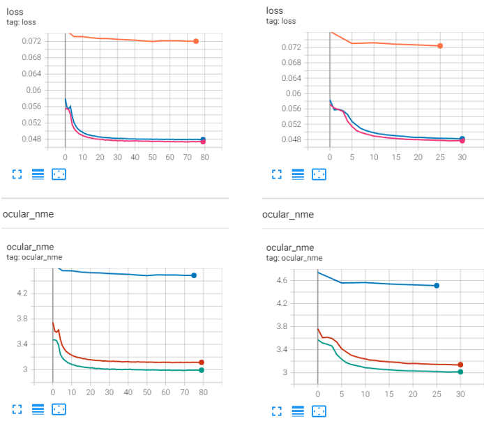
There is no significant difference in the effect of epochs on which you will freeze the quantization parameters(observers) and BatchNorm stats.

I tested various values of epoch to freeze the observers and bn stats, but there was no significant difference in the resulting converged value of loss or nme.

loss graph

pink : test loss before quantization
blue : training loss before quantization
orange : test loss after quantization

nme graph

green : test nme before quantization
red : training nme before quantization
blue : test nme after quantization

Exp 3. QAT - The effect of observer to calibrate the quantization parameters

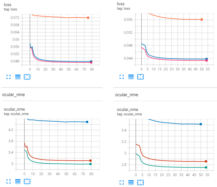
MovingAverageMinMaxObserver with U8S8 calibrated the quantization parameters(scale factor and zero-point integer) better than the default observer as shown in the graph below.

I tested only three kinds of observers : default observer, histogram observer, and MovingAverageMinMaxObserver with U8S8. Among them, the last one performed the best, but there are also many other types of observers and other observers may perform better. The observers are listed in the link below.

https://github.com/pytorch/pytorch/blob/main/torch/ao/quantization/observer.py

loss graph

pink : test loss before quantization
blue : training loss before quantization
orange : test loss after quantization

nme graph

green : test nme before quantization
red : training nme before quantization
blue : test nme after quantization

left : default observer
right : MovingAverageMinMaxObserver with U8S8

Experiment

dataset :
calibration : batch_size = 32, iteration = 32
inference : batch_size = 128, iteration = 61
hardware : cpu
learning rate : 1e-8

method	model size [MB]	inference time [s]	loss	ocualr_nme [%]	pupil_nme [%]
Original Model	44.011	76.06	0.04312033	2.73897	3.79658
Static PTQ with default observer	11.121	22.30	0.07286325	4.54174	6.29569
QAT with default observer	11.121	22.04	0.07202724	4.48688	6.21954
QAT with MovingAverage MinMaxObserver (U8S8)	11.121	21.75	0.05595706	3.50271	4.85493

Result

By both Post-Training Static Quantization and Quantization-Aware Training, model size of resnet18 was reduced by about 4 times.
By both Post-Training Static Quantization and Quantization-Aware Training, inference speed was improved by about 3.5 times.
QAT performs a little bit better than Static PTQ due to the fine-tuning process.
MovingAverageMinMaxObserver with U8S8 performed better than the default observer. However, there may exist another better observer since I only tested three kinds of observers.

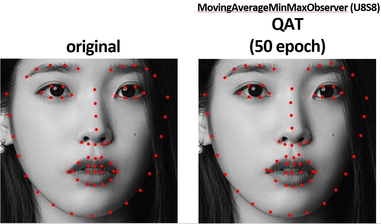
Generated landmark

You can see that the inference output of QAT model is better than that of Static PTQ model.

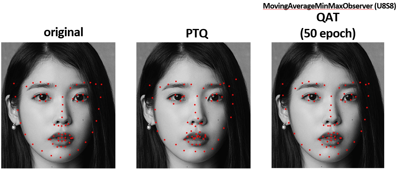
When the input is a tight face, the inference output of QAT model seems nearly similar to that of original model.

ONNX

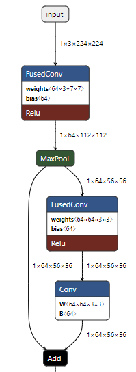
Visualization of ONNX via netron.app

Visualization of ONNX : Fused Model & Quantized Model (QDQ format)

INT8 Quantization of ONNX Runtime

INT8 Quantization follows the link below.

https://github.com/microsoft/onnxruntime-inference-examples/tree/main/quantization/image_classification/cpu

Experiment

dataset : inference : batch_size = 1, iteration = 7799
hardware : cpu

This table shows how I quantized each ONNX model adjusting combination of some parameters.

IN8 Quantization	freezed layer	per channel	reduce range	CalibTensor Range Symmetric	Calib Moving Average	Smooth Quant
Pre-processed Model
Quantized Model 1		T	F	T	T	T
Quantized Model 2		F	F	T	T	T
Quantized Model 3		T	F	F	T	T
Quantized Model 4		T	F	F	F	F
Quantized Model 5	fc layer	T	F	F	T	T
Quantized Model 6	ReLU & Add	T	F	F	T	T
Quantized Model 7	layer 4 & fc layer	T	F	F	T	T
Quantized Model 8	layer 4 & fc layer	T	T	F	T	T
Quantized Model 9	layer 4 & fc layer	T	T	F	T	T
Quantized Model 10	layer 4 & fc layer	T	T	F	T	T
Quantized Model 11	layer 1 & layer 4 & fc layer	T	T	F	T	T

INT8 Quantization	model size [MB]	inference time [s]	loss	ocualr_nme [%]	pupil_nme [%]
Pre-processed Model	44.044	83.05	0.00867057	2.73897	3.79658
Quantized Model 1	11.177	90.04	2.04831275	594.30187	823.93989
Quantized Model 2	11.113	91.34	2.08157768	603.68516	836.92611
Quantized Model 3	11.177	93.21	0.19241423	58.71200	81.41132
Quantized Model 4	11.177	90.74	0.20964802	65.31481	90.57096
Quantized Model 5	11.377	94.70	0.19232825	58.67378	81.35814
Quantized Model 6	11.226	100.37	0.19220746	58.66837	81.35119
Quantized Model 7	35.923	90.62	0.12938738	39.69218	55.05709
Quantized Model 8	35.923	87.56	0.12887142	39.57574	54.89788
Quantized Model 9	35.923	61.08	0.12887123	39.57566	54.89777
Quantized Model 10	35.923	60.07	0.12887123	39.57566	54.89777
Quantized Model 11	36.384	65.18	0.11555405	35.54718	49.31533

Result

By ONNX Quantization, model size of resnet18 was reduced by about 4 times for Quantized Model 1~6. (However, there is significant accuracy drop.)
By ONNX Quantization, there is no notable improvement on inference time.

The performance improvement depends on your model and hardware. The performance gain from quantization has two aspects: compute and memory. Old hardware has none or few of the instructions needed to perform efficient inference in int8. And quantization has overhead (from quantizing and dequantizing), so it is not rare to get worse performance on some devices.

x86-64 with VNNI, GPU with Tensor Core int8 support, and ARM with dot-product instructions can get better performance in general. But, there may not exist a notable improvement on inference time.
By ONNX Quantization, it is not rare to see significant accuracy drop. Then you can try U8U8.

When to try U8U8 data type? :

On x86-64 machines with AVX2 and AVX512 extensions, ONNX Runtime uses the VPMADDUBSW instruction for U8S8 for performance. However, this instruction might suffer from saturation issues: it can happen that the output does not fit into a 8-bit, 8-bit integer and has to be clamped (saturated) to fit. Generally, this is not a big issue for the final result. However, if you encounter a significant accuracy drop, it may be caused by saturation. In this case, you can try U8U8 with reduce_range.
By ONNX Quantization, it is not rare to see significant accuracy drop. Then you can try reduce_range = True or per_channel = True.

When to use reduce_range and per_channel quantization? :

Reduce-range will quantize the weights to 7-bits. It is designed for the U8S8 format on AVX2 and AVX512 (non-VNNI) machines to mitigate saturation issues. This is not needed on machines supporting VNNI.

Per-channel quantization can improve the accuracy for models whose weight ranges are large. You can try it if the accuracy drop is large. In addition, on AVX2 and AVX512 machines, you will generally need to enable reduce_range as well if per_channel is enabled.
By ONNX Quantization, it is not rare to see significant accuracy drop. To improve the problematic parts, you can compare the weights and activations tensors between the original computation graph and the quantized comptuation graph. By debugging, you can identify where they differ most and avoid quantizing these nodes.
I only tried ONNX Runtime quantization on CPU, but you can also try quantization on GPU and you can use many other Execution Providers.

The ONNX Runtime material below suggests that you can try quantization on GPU if there is a significant accuracy drop.

https://onnxruntime.ai/docs/performance/model-optimizations/quantization.html#quantization-on-gpu

If you are interested in other Execution Providers, refer to the link below.

https://onnxruntime.ai/docs/execution-providers/
If the Post-Training Quantization method cannot meet accuracy goal, you can try using QAT (Quantization-Aware Training) to retrain the model. However, ONNX Runtime does not provide retraining at this time, so you should re-train your models with the original framework (in my case, Pytorch) and convert them back to ONNX.

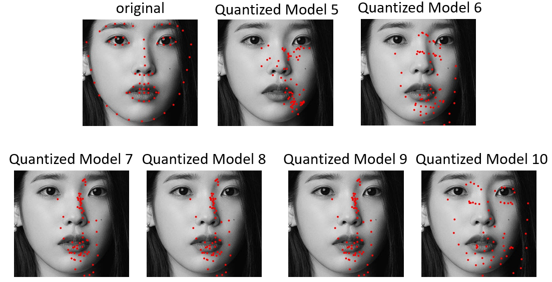
Generated landmark

You can see that accuracy drop of ONNX quantization is significant.

Debugging

Briefly, I will explain how to debug the weights of a model. To learn how to debug the activations of a model, refer to the link below.

https://github.com/microsoft/onnxruntime/blob/main/onnxruntime/python/tools/quantization/qdq_loss_debug.py

create_weight_matching("path/float.onnx", "path/qdq.onnx")
# This function dequantizes a quantized weight following
#	the linear dequantization equation x = s * (x_q - z)
# Then it returns dictA = {"onnx::Conv_193" : 
#					 									 {"float": w1, "dequantized" : w2},
#											 		 "onnx::Conv_194" : 
#														 {"float": w1, "dequantized" : w2}}
# Here, w1 means the fp32 weight of original model
# and w2 means the dequantized weight of quantized model

compute_weight_error(dictA)
# This function computes SQNR = P_signal / P_noise 
#                             = 20log(|w1|/|w1-w2|)
# Then it returns dictB = {"onnx::Conv_193" : SQNR1,
#                          "onnx::Conv_194" : SQNR2}
# If the SQNR value is larger, then it means the error is smaller.

By using the above functions, you can figure out which node has the significant quantization error and avoid quantizing those nodes.

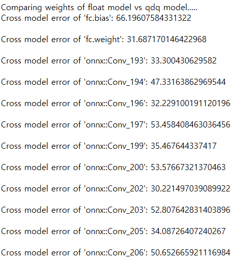
SQNR of each node by debugging

In my case, SQNR value for weight matrix of each node was in the range of [23, 37], which means that the value of \(\frac{\vert w1 \vert}{\vert w1-w2 \vert}\) is in the range of [14, 70].

Also, SQNR value for bias vector of each node was in the range of [46, 71], which means that the value of \(\frac{\vert w1 \vert}{\vert w1-w2 \vert}\) is in the range of [199, 3548].

FP16 Conversion of ONNX Runtime

FP16 Conversion follows the link below.

https://onnxruntime.ai/docs/performance/model-optimizations/float16.html

ONNX Runtime INT8 Quantization was not successful, so I also tried FP16 Conversion of an ONNX model.

Experiment

hardware : cpu

FP16 Conversion	model size [MB]	inference time [s]	loss	ocualr_nme [%]	pupil_nme [%]
Original Model	43.922	207.34	0.00867057	2.73897	3.79658
Converted Model	21.969	190.82	0.00867078	2.73904	3.79668

Result

By ONNX Runtime FP16 Conversion, the model size of resnet18 was reduced by about 2 times.
By ONNX Runtime FP16 Conversion on CPU, there was no notable improvement on inference time since CPU cannot utilize FP16 speedup. However, the inference speed will be improved if you use GPUs.
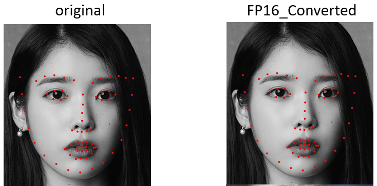
Accuracy drop almost does not occur after FP16 Conversion.

Generated landmark

Conclusion

In conclusion, I provided a comprehensive overview of the diverse quantization techniques available in Pytorch and ONNX. We have mainly discussed three techniques : Post-Training Dynamic Quantization, Post-Training Static Quantization, and Quantization-Aware Training.

Remember that quantization is required to efficiently deploy your model on resouce-constrained devices even if there is a trade-off of accuracy drop. Therefore, quantization has to be done targeting your specific hardware and there are actually various quantization details depending on the hardware. Starting with studying quantization in Pytorch and ONNX, I encourage you to dive deeper into quantization that fits your hardware.

Moreover, as the field of deep learning continues to expand, quantization will persist as a critical factor for the widespread deployment of neural network models on various hardware platforms and real-world applications. Therefore, I encourage you to continuously have interest in performance improvement including quantization so that you can successfully bridge the gap between powerful AI models and resource-constrained real-world environments.